In this article, we demonstrate a technique to derive the name of a worksheet within a cell in Excel. It uses a technique that is demonstrated in some of our teaching modules, using the TEXTAFTER and CELL functions.
A common request is to link the name of a worksheet with the value in a cell. It is frequently the case that the model or analysis designer wishes to provide the user the option to select an entry from a drop-down list and have that entry drive the logic in the worksheet and it seems obvious that the renaming of the worksheet to match the entry would be advisable. The entry selected may represent a product, territory, customer class, store, security code, property or some other member of a set of items to be forecast or analysed.
Without recourse to VBA or add-in programming, the request cannot be met using standard functionality and formulas in a cell. However, if you change the cause and effect, so that the naming of the sheet would trigger the changing of a value in a cell, and that entry then drives the logic in the worksheet, this is entirely achievable. Using the CELL function to derive the path to the worksheet, and the TEXTAFTER function to extract the worksheet name, this is now very simple.
One of the advantages of the TEXTAFTER function, is that it neatly solves the problem arising in the cases where the server supports the use of brackets in the path, so finding the text after the last bracket was messy in the past.
Simple Method - Using the Relatively New TEXTAFTER Function
To return the name of a worksheet in a cell, enter the following formula into the cell., replacing celladdress with the address of the cell into which the formula is added.
=TEXTAFTER(CELL("filename",celladdress),"]",-1)
NB: If the file has not yet been saved, so there is no valid path to its location, the formula will return #VALUE!.
Referring to the cell itself does not create a circular reference, since the cell's value depends upon its location, not its own value! Referring to the cell itself avoids errors arising if it referred to another cell, which was later deleted.
In the TEXTAFTER function, the instance_num is given as -1, meaning the function looks for the first "]" from the right-hand end of the text string returned by the CELL function.
See Also: LAMBDA Library: WorksheetName article.
Old Methods - Used Before TEXTAFTER was Available
These solutions are no longer required, if you have access to the TEXTAFTER function, the solution above is simpler and cleaner. But you may have older workbooks using these methods, so it is shown for comparison.
Assuming no ] Characters in Path
This required us to find the "]" in the string returned by the CELL function using the FIND function and then return the characters from the end of the string using the RIGHT function. The number of characters is calculated as the difference between the string's length calculated with the LEN function and the position of the "]" found by the FIND function.
To avoid redundantly calculating the worksheet's path over and over, this is calculated in two steps.
into one cell, enter the formula shown, replacing celladdress with the address of the cell into which the formula is added.
=CELL("filename",celladdress)
into a separate cell, enter the formula shown, replacing firstcelladdress with the address of the cell into which the previous formula was entered.
=RIGHT(firstcelladdress,LEN(firstcelladdress)-FIND("]",firstcelladdress))
Allowing for the Path to Contain ] Characters
The logic deployed in the previous example assumes that the workbook is not in a path that itself includes the square bracket characters. It would be unusual, and Excel will give you grief saving files into a directory that includes [] characters. But it can be the case, and sometimes also happens with download paths, either with square brackets added to the file name, or in the download path. So it is not sufficient to find the first ] character and assume that everything that follows is the worksheet name. I have created a path, and it has a valid Excel workbook, and the return value from the CELL function is: C:\Users\James Clarkson\Desktop\Test [with brackets]\[Book2.xlsx]Sheet1.
If I used the old formula pair given above, it would return the sheet name as "\[Book2.xlsx]Sheet1" - Not so good. Therefore, we need to modify the formula to be all the text after the last ].
To avoid redundantly calculating the worksheet's path over and over, this is calculated in two steps.
into one cell, enter the formula shown, replacing celladdress with the address of the cell into which the formula is added.
=CELL("filename",celladdress)
into a separate cell, enter the formula shown, replacing firstcelladdress with the address of the cell into which the previous formula was entered. This formula derives the count of ] characters in the path returned in the previous cell. It does this by deriving the length of the path using the LEN function, and then deriving the length of a modified copy created by the SUBSTITUTE function, in which the "]" characters are replaced with an empty string "", effectively removing them from the original string The value returned is the difference in lengths of the string that includes the brackets and the one that doesn't, therefore the nuber of brackets!
=LEN(firstcelladdress)-LEN(SUBSTITUTE(firstcelladdress ,"]",""))
into a third separate cell, enter the formula shown, replacing firstcelladdress with the address of the cell into which the first formula was entered and the formula was replacing secondcelladdress with the address of the cell into which the second formula was entered
=RIGHT(firstcelladdress,LEN(firstcelladdress)-FIND(CHAR(182),SUBSTITUTE(firstcelladdress,"]",CHAR(182),secondcelladdress)))
The CHAR(182) embedded in this formula returns the paragraph mark character (¶). This is used to provide a unique character to be found, avoiding any clash with the actual characters used in the path and worksheet name.
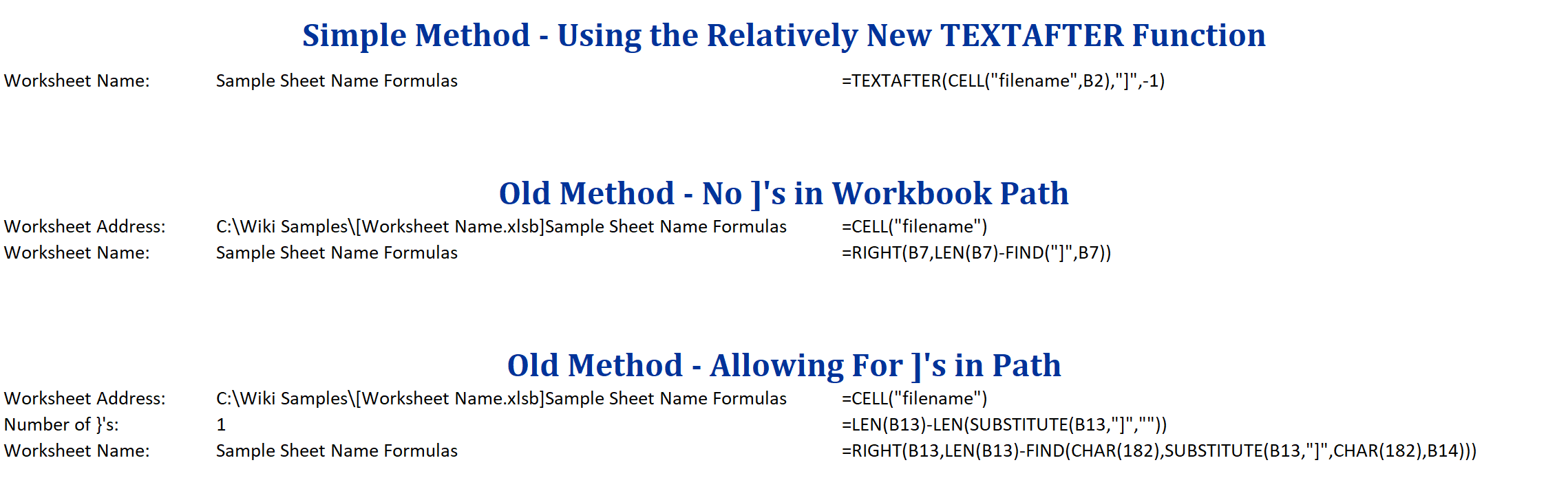 screenshot from the sample workbook, showing the formulas as described above
Open/download the sample workbook: Worksheet-Name.xlsb